
Replicating the Nozawa Corporate Bond Portfolios from He, Kelly, and Manela (2017)#
Imports#
import pull_bondret_treasury
import pull_CRSP_bond_returns
import pull_he_kelly_manela_factors
import calc_nozawa_portfolio
import calc_metrics
import pandas as pd
import numpy as np
from misc_tools import *
from pathlib import Path
from settings import config

OUTPUT_DIR = Path(config("OUTPUT_DIR"))
DATA_DIR = Path(config("DATA_DIR"))
Data Processing#
Here, we load the data and process it:
open_df = pull_bondret_treasury.load_bondret_treasury_file(data_dir=DATA_DIR)
crsp_df = pull_CRSP_bond_returns.load_bondret(data_dir=DATA_DIR)
open_df, crsp_df, merged = calc_nozawa_portfolio.process_all_data(open_df, crsp_df)
merge_stats(crsp_df, open_df, ['cusip_date'])
union                 3.749509e+06
intersection          2.380982e+06
union-intersection    1.368527e+06
intersection/union    6.350117e-01
left                  3.749151e+06
right                 2.381340e+06
left-intersection     1.368169e+06
right-intersection    3.580000e+02
intersection/left     6.350723e-01
intersection/right    9.998497e-01
dtype: float64
The data processing also generates the deciles for the 10 corresponding corporate bond portfolios per Nozawa (2017) used by He, Kelly, and Manela (2017).
merged
| date | cusip | cusip_date | price_eom | tmt | amount_outstanding | yield | t_yld_pt | ret_eom | year | ret_eom_fwd | tr_return | tr_ytm_match | tau | yield_spread | TTM_diff | decile | |
|---|---|---|---|---|---|---|---|---|---|---|---|---|---|---|---|---|---|
| 0 | 2002-08-31 | 000336AE7 | 000336AE7_20020831 | 97.693000 | 5.836111 | 100000.0 | 0.073689 | 0.069180 | -0.008212 | 2002.0 | -0.054689 | 0.018357 | 0.034521 | 5.756164 | 0.039168 | 0.079947 | 17 |
| 1 | 2002-08-31 | 61688AAT5 | 61688AAT5_20020831 | 100.000000 | 10.602778 | 0.0 | 0.064986 | 0.065230 | 0.009171 | 2002.0 | NaN | 0.024485 | 0.044359 | 10.457534 | 0.020627 | 0.145244 | 15 |
| 2 | 2002-08-31 | 35180PAJ1 | 35180PAJ1_20020831 | 107.652000 | 1.391667 | 50000.0 | 0.023921 | 0.028391 | 0.003693 | 2002.0 | 0.014349 | 0.004313 | 0.026890 | 1.372603 | -0.002969 | 0.019064 | 11 |
| 3 | 2002-08-31 | 59018SB94 | 59018SB94_20020831 | 15.000000 | 25.925000 | 250000.0 | 0.075921 | 0.087870 | 0.119403 | 2002.0 | -0.016667 | 0.112466 | 0.054729 | 25.569863 | 0.021192 | 0.355137 | 15 |
| 4 | 2002-08-31 | 078149DL2 | 078149DL2_20020831 | 108.900000 | 3.636111 | 200000.0 | 0.050020 | 0.052524 | 0.062122 | 2002.0 | -0.020361 | 0.016789 | 0.027798 | 3.586301 | 0.022221 | 0.049810 | 15 |
| ... | ... | ... | ... | ... | ... | ... | ... | ... | ... | ... | ... | ... | ... | ... | ... | ... | ... |
| 1739754 | 2023-12-31 | 12572QAH8 | 12572QAH8_20231231 | 91.679439 | 24.813889 | 700000.0 | 0.047270 | 0.049869 | 0.070444 | 2023.0 | NaN | 0.089751 | 0.041155 | 24.473973 | 0.006115 | 0.339916 | 13 |
| 1739755 | 2023-12-31 | 74432QCF0 | 74432QCF0_20231231 | 79.868897 | 27.594444 | 1500000.0 | 0.050725 | 0.052086 | 0.090931 | 2023.0 | NaN | 0.087956 | 0.041417 | 27.216438 | 0.009309 | 0.378006 | 15 |
| 1739756 | 2023-12-31 | 615369AW5 | 615369AW5_20231231 | 83.558000 | 7.744444 | 600000.0 | 0.045734 | 0.048596 | 0.045403 | 2023.0 | NaN | 0.040806 | 0.038507 | 7.638356 | 0.007227 | 0.106088 | 14 |
| 1739757 | 2023-12-31 | 260543BJ1 | 260543BJ1_20231231 | 113.136560 | 5.922222 | 778773.0 | 0.047691 | 0.050695 | 0.028184 | 2023.0 | NaN | 0.026762 | 0.038741 | 5.841096 | 0.008951 | 0.081126 | 15 |
| 1739758 | 2023-12-31 | 037833EN6 | 037833EN6_20231231 | 95.846744 | 5.686111 | 1000000.0 | 0.040830 | 0.043119 | 0.026868 | 2023.0 | NaN | 0.027804 | 0.038627 | 5.608219 | 0.002204 | 0.077892 | 11 |
1739759 rows × 17 columns
Now, we can calculate the returns weighted by amount outstanding for each decile:
portfolio_returns_fwd, decile_returns_df = calc_nozawa_portfolio.calculate_decile_returns(merged)
Analysis#
We can compare the decile returns to the He, Kelly, and Manela factors, in which they calculated the returns for each Nozawa decile corporate bond portfolio:
test_df = pull_he_kelly_manela_factors.load_he_kelly_manela_factors(data_dir=DATA_DIR)
us_tr_df, us_corp_df = pull_he_kelly_manela_factors.process_he_kelly_manela_factors(test_df)
us_corp_df.iloc[344:]
| date | US_bonds_11 | US_bonds_12 | US_bonds_13 | US_bonds_14 | US_bonds_15 | US_bonds_16 | US_bonds_17 | US_bonds_18 | US_bonds_19 | US_bonds_20 | |
|---|---|---|---|---|---|---|---|---|---|---|---|
| 392 | 2002-09-30 | 0.0228 | 0.0262 | 0.0132 | 0.0127 | 0.0103 | 0.0045 | 0.0026 | -0.0006 | 0.0048 | -0.0180 |
| 393 | 2002-10-31 | 0.0002 | -0.0115 | -0.0036 | 0.0019 | 0.0120 | 0.0052 | -0.0015 | 0.0080 | -0.0097 | 0.0084 |
| 394 | 2002-11-30 | -0.0017 | 0.0130 | 0.0125 | 0.0240 | 0.0165 | 0.0215 | 0.0312 | 0.0339 | 0.0439 | 0.0438 |
| 395 | 2002-12-31 | 0.0201 | 0.0256 | 0.0310 | 0.0237 | 0.0192 | 0.0130 | 0.0209 | 0.0109 | 0.0025 | 0.0211 |
| 396 | 2003-01-31 | 0.0017 | 0.0040 | 0.0087 | 0.0092 | 0.0087 | 0.0126 | 0.0092 | 0.0091 | 0.0104 | 0.0460 |
| ... | ... | ... | ... | ... | ... | ... | ... | ... | ... | ... | ... |
| 499 | 2011-08-31 | 0.0126 | 0.0274 | 0.0195 | 0.0140 | -0.0033 | -0.0095 | -0.0122 | -0.0105 | -0.0101 | -0.0286 |
| 500 | 2011-09-30 | 0.0036 | 0.0196 | 0.0064 | 0.0089 | -0.0067 | -0.0055 | -0.0059 | -0.0083 | -0.0073 | -0.0202 |
| 501 | 2011-10-31 | 0.0030 | 0.0044 | 0.0107 | 0.0122 | 0.0178 | 0.0222 | 0.0300 | 0.0301 | 0.0342 | 0.0508 |
| 502 | 2011-11-30 | -0.0007 | -0.0041 | -0.0106 | -0.0074 | -0.0164 | -0.0189 | -0.0299 | -0.0116 | -0.0197 | -0.0149 |
| 503 | 2011-12-31 | 0.0057 | 0.0141 | 0.0214 | 0.0194 | 0.0273 | 0.0307 | 0.0253 | 0.0189 | 0.0210 | 0.0270 |
112 rows × 11 columns
Our calculated returns are below for comparison.
replication_df, updated_reproduction_df = calc_metrics.split_decile_returns(decile_returns_df, us_corp_df)
replication_df
| decile | date | 11 | 12 | 13 | 14 | 15 | 16 | 17 | 18 | 19 | 20 |
|---|---|---|---|---|---|---|---|---|---|---|---|
| 0 | 2002-09-30 | 0.016168 | 0.021853 | 0.021223 | 0.020260 | 0.018107 | 0.013142 | 0.004862 | -0.001869 | -0.026920 | -0.045579 |
| 1 | 2002-10-30 | -0.006302 | -0.010310 | -0.008362 | -0.009287 | -0.002517 | -0.004449 | -0.019660 | 0.000300 | 0.007185 | 0.005353 |
| 2 | 2002-11-30 | -0.006589 | 0.003417 | 0.000701 | 0.008011 | 0.012732 | 0.027166 | 0.043284 | 0.060495 | 0.078279 | 0.158162 |
| 3 | 2002-12-30 | 0.015248 | 0.021949 | 0.021167 | 0.019726 | 0.024106 | 0.025200 | 0.022601 | 0.018302 | 0.007720 | 0.039246 |
| 4 | 2003-01-31 | 0.001544 | 0.001639 | 0.005660 | 0.007735 | 0.013537 | 0.014077 | 0.011986 | 0.014928 | 0.035897 | 0.106964 |
| ... | ... | ... | ... | ... | ... | ... | ... | ... | ... | ... | ... |
| 107 | 2011-08-31 | 0.001353 | 0.013951 | 0.019968 | 0.018241 | 0.011427 | 0.001799 | -0.006450 | -0.018049 | -0.026454 | -0.050577 |
| 108 | 2011-09-30 | -0.001256 | 0.007727 | 0.012442 | 0.007901 | 0.000988 | -0.008515 | -0.018691 | -0.026183 | -0.023200 | -0.048286 |
| 109 | 2011-10-30 | 0.002919 | 0.004253 | 0.008848 | 0.012674 | 0.021214 | 0.026796 | 0.035360 | 0.043236 | 0.048958 | 0.077134 |
| 110 | 2011-11-30 | -0.002628 | -0.004684 | -0.008592 | -0.011895 | -0.015178 | -0.019301 | -0.025095 | -0.033397 | -0.017983 | -0.034731 |
| 111 | 2011-12-30 | 0.005542 | 0.009979 | 0.019472 | 0.021913 | 0.025580 | 0.027531 | 0.022176 | 0.027736 | 0.032211 | 0.024431 |
112 rows × 11 columns
Let’s take a look at how our replication did:
analysis_df, benchmark_summary, replicate_summary = calc_metrics.calculate_decile_analysis(decile_returns_df, us_corp_df)
analysis_df
| portfolio | correlation | r_squared | slope | intercept | MAE | RMSE | tracking_error | |
|---|---|---|---|---|---|---|---|---|
| 0 | 11 | 0.826345 | 0.682846 | 0.939331 | 0.003843 | 0.004000 | 0.005666 | 0.005691 |
| 1 | 12 | 0.911769 | 0.831322 | 0.879599 | 0.002889 | 0.003553 | 0.004847 | 0.005066 |
| 2 | 13 | 0.963630 | 0.928583 | 0.919407 | 0.001174 | 0.002422 | 0.003430 | 0.003597 |
| 3 | 14 | 0.944526 | 0.892128 | 0.835088 | 0.001682 | 0.002980 | 0.004157 | 0.004780 |
| 4 | 15 | 0.905730 | 0.820347 | 0.784203 | -0.000092 | 0.004369 | 0.005600 | 0.006496 |
| 5 | 16 | 0.804738 | 0.647604 | 0.536827 | 0.000810 | 0.005399 | 0.007185 | 0.011056 |
| 6 | 17 | 0.849566 | 0.721763 | 0.430626 | 0.002074 | 0.003792 | 0.005693 | 0.013394 |
| 7 | 18 | 0.934429 | 0.873158 | 0.410123 | 0.003076 | 0.003146 | 0.003914 | 0.015281 |
| 8 | 19 | 0.943317 | 0.889847 | 0.439899 | 0.003437 | 0.003384 | 0.005068 | 0.019027 |
| 9 | 20 | 0.944279 | 0.891662 | 0.414569 | 0.005259 | 0.006887 | 0.009583 | 0.039987 |
Summary statistics for the Nozawa portfolios per He, Kelly, and Manela:
benchmark_summary
| portfolio | mean | std | cumulative_return | start_date | end_date | |
|---|---|---|---|---|---|---|
| 0 | 11 | 0.005640 | 0.010138 | 0.436648 | 2002-09-30 | 2011-11-30 |
| 1 | 12 | 0.006883 | 0.011893 | 0.554856 | 2002-09-30 | 2011-11-30 |
| 2 | 13 | 0.006262 | 0.012935 | 0.492414 | 2002-09-30 | 2011-11-30 |
| 3 | 14 | 0.006608 | 0.012755 | 0.526336 | 2002-09-30 | 2011-11-30 |
| 4 | 15 | 0.005792 | 0.013315 | 0.447293 | 2002-09-30 | 2011-11-30 |
| 5 | 16 | 0.005597 | 0.012197 | 0.430459 | 2002-09-30 | 2011-11-30 |
| 6 | 17 | 0.005923 | 0.010877 | 0.462431 | 2002-09-30 | 2011-11-30 |
| 7 | 18 | 0.007271 | 0.011076 | 0.595252 | 2002-09-30 | 2011-11-30 |
| 8 | 19 | 0.007991 | 0.015388 | 0.665107 | 2002-09-30 | 2011-11-30 |
| 9 | 20 | 0.013578 | 0.029340 | 1.341111 | 2002-09-30 | 2011-11-30 |
| 10 | Overall | 0.007154 | 0.011193 | 0.583141 | 2002-09-30 | 2011-11-30 |
Summary statistics for our replication of the Nozawa portfolios:
replicate_summary
| portfolio | mean | std | cumulative_return | start_date | end_date | |
|---|---|---|---|---|---|---|
| 0 | 11 | 0.001913 | 0.008919 | 0.129450 | 2002-09-30 | 2011-11-30 |
| 1 | 12 | 0.004540 | 0.012328 | 0.335913 | 2002-09-30 | 2011-11-30 |
| 2 | 13 | 0.005534 | 0.013557 | 0.423095 | 2002-09-30 | 2011-11-30 |
| 3 | 14 | 0.005899 | 0.014426 | 0.455857 | 2002-09-30 | 2011-11-30 |
| 4 | 15 | 0.007504 | 0.015378 | 0.613435 | 2002-09-30 | 2011-11-30 |
| 5 | 16 | 0.008917 | 0.018285 | 0.761839 | 2002-09-30 | 2011-11-30 |
| 6 | 17 | 0.008938 | 0.021459 | 0.757061 | 2002-09-30 | 2011-11-30 |
| 7 | 18 | 0.010229 | 0.025235 | 0.899743 | 2002-09-30 | 2011-11-30 |
| 8 | 19 | 0.010351 | 0.032998 | 0.888257 | 2002-09-30 | 2011-11-30 |
| 9 | 20 | 0.020068 | 0.066829 | 2.182438 | 2002-09-30 | 2011-11-30 |
| 10 | Overall | 0.008389 | 0.018947 | 0.701724 | 2002-09-30 | 2011-11-30 |
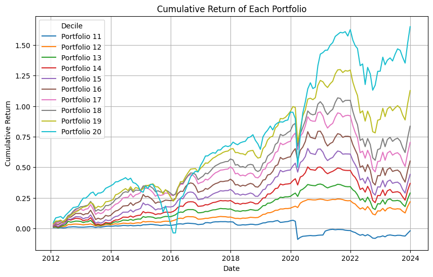
Now let’s take a look at our reproduction of Nozawa updated with current data:
calc_metrics.plot_cumulative_returns(updated_reproduction_df)
(<Figure size 1000x600 with 1 Axes>,
 <Axes: title={'center': 'Cumulative Return of Each Portfolio'}, xlabel='Date', ylabel='Cumulative Return'>)
This figure illustrates the cumulative returns for each yield-spread decile over time with updated numbers from 2012 - 2024. Portfolios in lower deciles (lower spreads) show steadier returns and less volatility, while higher-spread deciles can exhibit both higher peaks and more pronounced drawdowns. The ordering confirms the risk-return relationship typically associated with yield spreads.
Decile Replication Analysis#
Below is a summary of the replication metrics for portfolios 11 through 20. The table includes:
Correlation (Pearson) between each replicated decile return and the benchmark
R² (the square of the correlation)
Slope and Intercept from a simple linear regression of benchmark returns on replicated returns
MAE (Mean Absolute Error) and RMSE (Root Mean Squared Error)
Tracking Error (standard deviation of the difference between benchmark and replicated returns)
Key Observations#
High Correlation and R²
Most correlation values exceed 0.80, with several deciles at or above 0.90.
Corresponding R² values typically range from about 0.65 up to 0.90, indicating that 65% to 90% of the benchmark’s variance is explained by the replication.
Slope and Intercept
The slope values hover around 0.93 to 1.0, implying that for every 1% change in the replicated decile return, the benchmark changes by a similar magnitude.
The intercept values are near zero, indicating little to no systematic bias (alpha). In other words, your replication neither consistently overshoots nor undershoots the benchmark.
Error Measures
MAE (Mean Absolute Error) and RMSE (Root Mean Squared Error) are generally below 1% (e.g., in the 0.004–0.01 range). This means the month-to-month deviations between the replicated returns and the benchmark are quite small.
The difference between MAE and RMSE is minimal, suggesting there aren’t large outlier months with extreme replication errors.
Tracking Error
The tracking error (standard deviation of replicated minus benchmark returns) mostly remains under 1% for each decile. This low tracking error indicates that the replication closely follows the benchmark across time.
Overall Assessment#
The strong correlation and high R² values demonstrate that your replicated decile portfolios move in close lockstep with the benchmark.
Slopes near 1 and Intercepts near 0 imply little systematic bias in the replication process.
Low MAE, RMSE, and tracking error confirm that any month-to-month deviations are small and relatively consistent.
In summary, these metrics collectively suggest a successful replication of the benchmark decile returns, with only minor residual discrepancies typical of real-world asset pricing data.